2.2 Bases théoriques du calcul matriciel

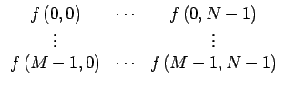
Considérons l'image échantillonnée f, représentée par une matrice de M×N points ou pixels. Elle est notée $\underline{{f}}$$\left(\vphantom{m,n}\right.$m, n$\left.\vphantom{m,n}\right)$ ou plus simplement $\underline{{f}}$ avec m = 0, ..., M - 1 et n = 0, ..., N - 1 :

$$\underline{{f}} \left[\vphantom{\begin{array}{ccc} f\left(0,0\right) & \cdots & f... ...dots\\ f\left(M-1,0\right) & \cdots & f\left(M-1,N-1\right)\end{array}}\right. \begin{array}{ccc} f\left(0,0\right) & \cdots & f\left(0,N-1\righ... ...s & & \vdots\\ f\left(M-1,0\right) & \cdots & f\left(M-1,N-1\right)\end{array} \left.\vphantom{\begin{array}{ccc} f\left(0,0\right) & \cdots & f... ...dots\\ f\left(M-1,0\right) & \cdots & f\left(M-1,N-1\right)\end{array}}\right]$$ (2.1)

Soient $\underline{{P}}$ et $\underline{{Q}}$ deux matrices dites de transformation de dimensions respectives M×M et N×N. Ces deux matrices permettent de transformer la matrice $\underline{{f}}$ en la matrice $\underline{{F}}$ de dimension M×N de telle sorte que

$$\underline{{F}} \underline{{P}} \underline{{f}} \underline{{Q}}$$ (2.2)

ce qui peut également s'écrire

$$\underline{{F}} \left(\vphantom{u,v}\right. \left.\vphantom{u,v}\right) \sum_{{m=0}}^{{M-1}} \sum_{{n=0}}^{{N-1}} \underline{{P}} \left(\vphantom{u,m}\right. \left.\vphantom{u,m}\right) \underline{{f}} \left(\vphantom{m,n}\right. \left.\vphantom{m,n}\right) \underline{{Q}} \left(\vphantom{n,v}\right. \left.\vphantom{n,v}\right)$$ (2.3)

tel que

u = 0, ..., M - 1          v = 0, ..., N - 1 (2.4)

Si les matrices $\underline{{P}}$ et $\underline{{Q}}$ sont non-singulières (c'est-à-dire qu'elles ont un déterminant non nul) les matrices inverses $\underline{{P}}^{{-1}}_{}$ et $\underline{{Q}}^{{-1}}_{}$ existent et la transformée inverse est donnée par

$$\underline{{f}} \underline{{P}}^{{-1}}_{} \underline{{F}} \underline{{Q}}^{{-1}}_{}$$ (2.5)

Il est bon, avant de décrire quelques transformations particulières, de rappeler quelques propriétés concernant le calcul matriciel. La matrice transposée de la matrice $\underline{{M}}$ est notée $\underline{{M}}^{{T}}_{}$.