Il existe 4 définitions de la transformée en cosinus discrète, parfois notées DCT-1, DCT-2, DCT-3, et DCT-4. Ces définitions diffèrent par les conditions limites qu'elles imposent aux bords2.1.
La transformée la plus utilisée en traitement et compression d'images est la DCT-2 dont la définition suit. D'un point de vue théorique, cette variante présuppose que l'image a été miroirisée le long de ses bords car, dans ce cas, la transformée de FOURIER de la séquence miroirisée est rigoureusement égale à la DCT-2 de la séquence originale.
Nous faisons l'hypothèse que l'image est carrée de dimension N×N.
Soit la matrice de transformation
![]()
![]() k, l
k, l![]() définie par
définie par
![$\displaystyle \begin{array}{ccc} \frac{1}{\sqrt{N}} & & l=0\\ \sqrt{\frac{2}{N}}\cos\left[\frac{\left(2k+1\right)l\pi}{2N}\right] & & sinon\end{array}$](img216.gif) |
(2.26) |
Une autre forme pour la transformée en cosinus discrète est donnée par
  u u v v |
(2.28) |
| u = 0, 1, ..., N - 1 v = 0, 1, ..., N - 1 | (2.29) |
c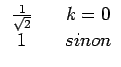 |
(2.30) |
| uv |
(2.31) |
| m = 0, 1, ..., N - 1 n = 0, 1, ..., N - 1 | (2.32) |