Table des matières of 2.7.1 Impulsion de DIRAC bidimensionnelle

2.7.1 Impulsion de DIRAC bidimensionnelle

Définition 7 La fonction delta ou impulsion de DIRAC bidimensionnelle , notée $\delta$ $\left(\vphantom{x,y}\right.$ x, y $\left.\vphantom{x,y}\right)$ , est définie par

$\displaystyle \delta$ $\displaystyle \left(\vphantom{x,y}\right.$ x, y $\displaystyle \left.\vphantom{x,y}\right)$ = 0 $\displaystyle \forall$ $\displaystyle \left(\vphantom{x,y}\right.$ x, y $\displaystyle \left.\vphantom{x,y}\right)$ $\displaystyle \neq$ $\displaystyle \left(\vphantom{0,0}\right.$ 0, 0 $\displaystyle \left.\vphantom{0,0}\right)$

(2.69)

$\displaystyle \int_{{-\infty}}^{{+\infty}}$ $\displaystyle \int_{{-\infty}}^{{+\infty}}$ $\displaystyle \delta$ $\displaystyle \left(\vphantom{x,y}\right.$ x, y $\displaystyle \left.\vphantom{x,y}\right)$ dxdy = 1

(2.70)

Il est possible de donner une autre définition équivalente de l'impulsion de DIRAC qui englobe les équations 2.69 et 2.70

$\displaystyle \int_{{-\infty}}^{{+\infty}}$ $\displaystyle \int_{{-\infty}}^{{+\infty}}$ f $\displaystyle \left(\vphantom{x,y}\right.$ x, y $\displaystyle \left.\vphantom{x,y}\right)$ $\displaystyle \delta$ $\displaystyle \left(\vphantom{x-\alpha,y-\beta}\right.$ x - $\displaystyle \alpha$ , y - $\displaystyle \beta$ $\displaystyle \left.\vphantom{x-\alpha,y-\beta}\right)$ dxdy = f $\displaystyle \left(\vphantom{\alpha,\beta}\right.$ $\displaystyle \alpha$ , $\displaystyle \beta$ $\displaystyle \left.\vphantom{\alpha,\beta}\right)$

(2.71)

où f $\left(\vphantom{x,y}\right.$ x, y $\left.\vphantom{x,y}\right)$ est une fonction continue de x et y.

2.7.1.1 Propriétés

La fonction $\delta$ $\left(\vphantom{x,y}\right.$ x, y $\left.\vphantom{x,y}\right)$ est spatialement séparable en deux fonctions de DIRAC à une dimension

$\displaystyle \delta$ $\displaystyle \left(\vphantom{x,y}\right.$ x, y $\displaystyle \left.\vphantom{x,y}\right)$ = $\displaystyle \delta$ $\displaystyle \left(\vphantom{x}\right.$ x $\displaystyle \left.\vphantom{x}\right)$ $\displaystyle \delta$ $\displaystyle \left(\vphantom{y}\right.$ y $\displaystyle \left.\vphantom{y}\right)$

(2.72)

Étant donné que la fonction $\delta$ $\left(\vphantom{x,y}\right.$ x, y $\left.\vphantom{x,y}\right)$ est une fonction symétrique par rapport à l'origine, l'équation (2.71) peut encore s'écrire, en changeant les variables d'intégration, sous la forme

$\displaystyle \int_{{-\infty}}^{{+\infty}}$ $\displaystyle \int_{{-\infty}}^{{+\infty}}$ f $\displaystyle \left(\vphantom{\alpha,\beta}\right.$ $\displaystyle \alpha$ , $\displaystyle \beta$ $\displaystyle \left.\vphantom{\alpha,\beta}\right)$ $\displaystyle \delta$ $\displaystyle \left(\vphantom{x-\alpha,y-\beta}\right.$ x - $\displaystyle \alpha$ , y - $\displaystyle \beta$ $\displaystyle \left.\vphantom{x-\alpha,y-\beta}\right)$ d $\displaystyle \alpha$ d $\displaystyle \beta$ = f $\displaystyle \left(\vphantom{x,y}\right.$ x, y $\displaystyle \left.\vphantom{x,y}\right)$

(2.73)

Le membre de gauche de l'équation 2.73 représente le produit de convolution de f $\left(\vphantom{x,y}\right.$ x, y $\left.\vphantom{x,y}\right)$ par $\delta$ $\left(\vphantom{x,y}\right.$ x, y $\left.\vphantom{x,y}\right)$ . On peut donc écrire

f $\displaystyle \left(\vphantom{x,y}\right.$ x, y $\displaystyle \left.\vphantom{x,y}\right)$ $\displaystyle \otimes$ $\displaystyle \delta$ $\displaystyle \left(\vphantom{x,y}\right.$ x, y $\displaystyle \left.\vphantom{x,y}\right)$ = f $\displaystyle \left(\vphantom{x,y}\right.$ x, y $\displaystyle \left.\vphantom{x,y}\right)$

(2.74)

Dès lors, la convolution d'une fonction f $\left(\vphantom{x,y}\right.$ x, y $\left.\vphantom{x,y}\right)$ avec l'impulsion de DIRAC laisse cette fonction inchangée.

2.7.1.2 Transformée de FOURIER

Par définition, la transformée de FOURIER de $\delta$ $\left(\vphantom{x,y}\right.$ x, y $\left.\vphantom{x,y}\right)$ est donnée par

(2.75)

Étant donné que la fonction e^{-2jxu + yv} évaluée en l'origine $\left(\vphantom{0,0}\right.$ 0, 0 $\left.\vphantom{0,0}\right)$ vaut 1, il vient finalement

$\displaystyle \delta$ $\displaystyle \left(\vphantom{x,y}\right.$ x, y $\displaystyle \left.\vphantom{x,y}\right)$ $\displaystyle \rightleftharpoons$ 1

(2.76)

Donc, le spectre en fréquence de l'impulsion de DIRAC s'étend uniformément sur tout l'intervalle fréquentiel $\left[\vphantom{-\infty,+\infty}\right.$ - $\infty$ , + $\infty$ $\left.\vphantom{-\infty,+\infty}\right]$ × $\left[\vphantom{-\infty,+\infty}\right.$ - $\infty$ , + $\infty$ $\left.\vphantom{-\infty,+\infty}\right]$ .

2.7.1.3 Liens avec quelques images typiques

Image continue
En utilisant la propriété de dualité (relation 2.46) de la transformée de FOURIER et étant donné que $\delta$ $\left(\vphantom{x,y}\right.$ x, y $\left.\vphantom{x,y}\right)$ est symétrique par rapport à l'origine, on peut écrire

1 $\displaystyle \rightleftharpoons$ $\displaystyle \delta$ $\displaystyle \left(\vphantom{u,v}\right.$ u, v $\displaystyle \left.\vphantom{u,v}\right)$ (2.77)

Le spectre d'une image continue est donc discret et comporte une seule raie située à l'origine $\left(\vphantom{0,0}\right.$ 0, 0 $\left.\vphantom{0,0}\right)$ du plan u - v.
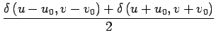
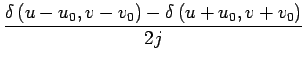
Image complexe exponentielle
En appliquant la propriété de translation fréquentielle (relation 2.48) de la transformée de FOURIER à 2.77, il vient

e^{-2ju₀x + v₀x} $\displaystyle \rightleftharpoons$ $\displaystyle \delta$ $\displaystyle \left(\vphantom{u-u_{0},v-v_{0}}\right.$ u - u₀, v - v₀ $\displaystyle \left.\vphantom{u-u_{0},v-v_{0}}\right)$ (2.78)

Le spectre d'une image complexe exponentielle de fréquence $\left(\vphantom{u_{0},v_{0}}\right.$ u₀, v₀ $\left.\vphantom{u_{0},v_{0}}\right)$ se limite donc à une raie située en $\left(\vphantom{u_{0},v_{0}}\right.$ u₀, v₀ $\left.\vphantom{u_{0},v_{0}}\right)$ dans le plan u - v.
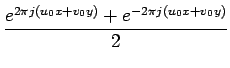
Image sinusoïdale
Soit l'image cos $\left[\vphantom{2\pi\left(u_{0}x+v_{0}y\right)}\right.$ 2 $\pi$ $\left(\vphantom{u_{0}x+v_{0}y}\right.$ u₀x + v₀y $\left.\vphantom{u_{0}x+v_{0}y}\right)$ $\left.\vphantom{2\pi\left(u_{0}x+v_{0}y\right)}\right]$ . Rappelons tout d'abord la formule bien connue

cos $\displaystyle \left[\vphantom{2\pi\left(u_{0}x+v_{0}y\right)}\right.$ 2 $\displaystyle \pi$ $\displaystyle \left(\vphantom{u_{0}x+v_{0}y}\right.$ u₀x + v₀y $\displaystyle \left.\vphantom{u_{0}x+v_{0}y}\right)$ $\displaystyle \left.\vphantom{2\pi\left(u_{0}x+v_{0}y\right)}\right]$ = $\displaystyle {\frac{{e^{2\pi j\left(u_{0}x+v_{0}y\right)}+e^{-2\pi j\left(u_{0}x+v_{0}y\right)}}}{{2}}}$ (2.79)

En utilisant la relation 2.78 et la propriété de linéarité de la transformée de FOURIER, il vient

cos $\displaystyle \left[\vphantom{2\pi\left(u_{0}x+v_{0}y\right)}\right.$ 2 $\displaystyle \pi$ $\displaystyle \left(\vphantom{u_{0}x+v_{0}y}\right.$ u₀x + v₀y $\displaystyle \left.\vphantom{u_{0}x+v_{0}y}\right)$ $\displaystyle \left.\vphantom{2\pi\left(u_{0}x+v_{0}y\right)}\right]$ $\displaystyle \rightleftharpoons$ $\displaystyle {\frac{{\delta\left(u-u_{0},v-v_{0}\right)+\delta\left(u+u_{0},v+v_{0}\right)}}{{2}}}$ (2.80)

Le spectre d'une image cosinusoïdale comporte donc 2 raies situées en $\left(\vphantom{u_{0},v_{0}}\right.$ u₀, v₀ $\left.\vphantom{u_{0},v_{0}}\right)$ et $\left(\vphantom{-u_{0},-v_{0}}\right.$ - u₀, - v₀ $\left.\vphantom{-u_{0},-v_{0}}\right)$ dans le plan u - v. Il est également aisé de montrer que

sin $\displaystyle \left[\vphantom{2\pi\left(u_{0}x+v_{0}y\right)}\right.$ 2 $\displaystyle \pi$ $\displaystyle \left(\vphantom{u_{0}x+v_{0}y}\right.$ u₀x + v₀y $\displaystyle \left.\vphantom{u_{0}x+v_{0}y}\right)$ $\displaystyle \left.\vphantom{2\pi\left(u_{0}x+v_{0}y\right)}\right]$ $\displaystyle \rightleftharpoons$ $\displaystyle {\frac{{\delta\left(u-u_{0},v-v_{0}\right)-\delta\left(u+u_{0},v+v_{0}\right)}}{{2j}}}$ (2.81)